LLM基础：Language Model & Transformer

 1. 什么是语言模型？

一句话，语言模型是这样一个模型：对于任意的词序列，它能够计算出这个序列是一句话的概率。

从文本生成角度来看，语言模型可以定义为：给定一个短语(一个词组或一句话)，语言模型可以生成(预测)接下来的一个词。

2. Transformer

Transformer 是谷歌大脑 2017 年论文《Attentnion is all you need》中提出的 seq2seq 模型，现已获得了大范围扩展和应用。而应用的方式主要是：先预训练语言模型，然后把预训练模型适配给下游任务，以完成各种不同任务，如分类、生成、标记等。

Transformer算法采用 self-attention 机制实现快速并行；此外，Transformer 还可以加深网络深度，不像 CNN 只能将模型添加到 2 至 3 层，这样它能够获取更多全局信息，进而提升模型准确率。

Transformer 结构

如下是用 Transformer 进行中英文翻译的示例图：

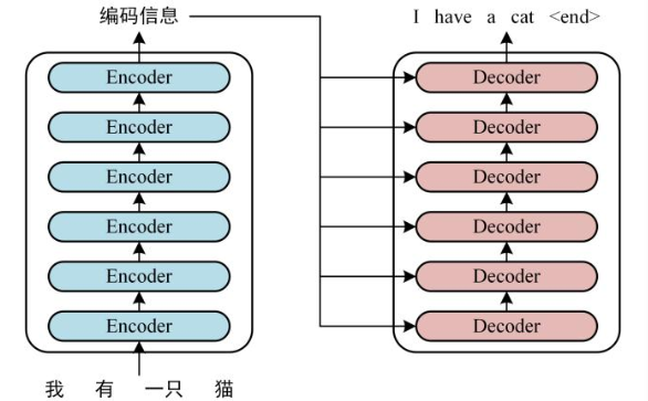
Transformer 由两大部分组成：编码器（Encoder） 和解码器（Decoder），每个模块都包含 6 个 block。所有的编码器在结构上都是相同的，负责把自然语言序列映射成为隐藏层，它们含有自然语言序列的表达式，但没有共享参数。然后解码器把隐藏层再映射为自然语言序列，从而解决各种 NLP 问题。

就上述示例而言，具体的实现可以分如下三步完成：

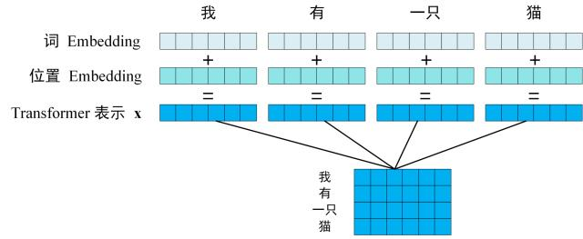
第一步：获取输入单词的词向量 X，X 由词嵌入和位置嵌入相加得到。其中词嵌入可以采用 Word2Vec 或 Transformer 算法预训练得到，也可以使用现有的 Tencent_AILab_ChineseEmbedding。

由于 Transformer 模型不具备循环神经网络的迭代操作，所以我们需要向它提供每个词的位置信息，以便识别语言中的顺序关系，因此位置嵌入非常重要。模型的位置信息采用 sin 和 cos 的线性变换来表达：

PE（pos,2i）=sin(pos/100002i/d)
PE (pos,2i+1)=cos(pos/100002i/d)

其中，pos 表示单词在句子中的位置，比如句子由 10 个词组成，则 pos 表示 [0-9] 的任意位置，取值范围是 [0,max sequence]；i 表示词向量的维度，取值范围 [0,embedding dimension]，例如某个词向量是 256 维，则 i 的取值范围是 [0-255]；d 表示 PE 的维度，也就是词向量的维度，如上例中的 256 维；2i 表示偶数的维度（sin）；2i+1 表示奇数的维度（cos）。

以上 sin 和 cos 这组公式，分别对应 embedding dimension 维度一组奇数和偶数的序号的维度，例如，0,1 一组，2,3 一组。分别用上面的 sin 和 cos 函数做处理，从而产生不同的周期性变化，学到位置之间的依赖关系和自然语言的时序特性。

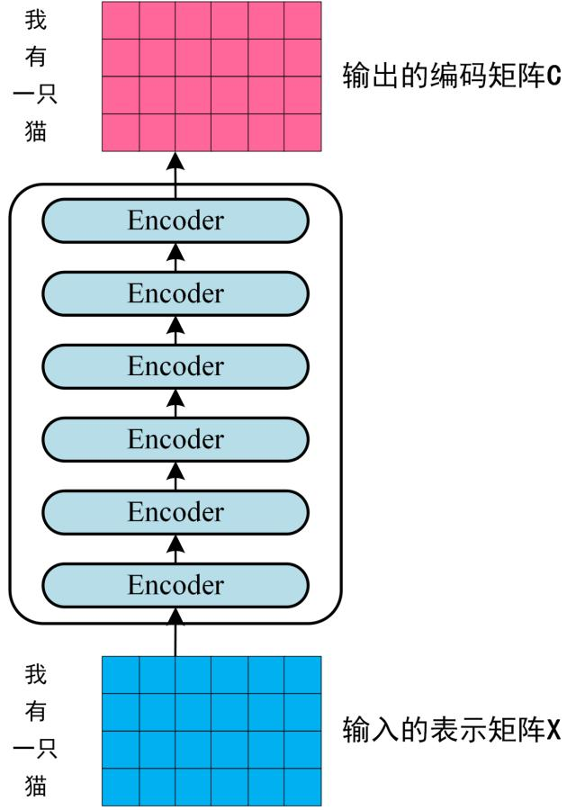
第二步：将第一步得到的向量矩阵传入编码器，编码器包含 6 个 block ，输出编码后的信息矩阵 C。每一个编码器输出的 block 维度与输入完全一致。

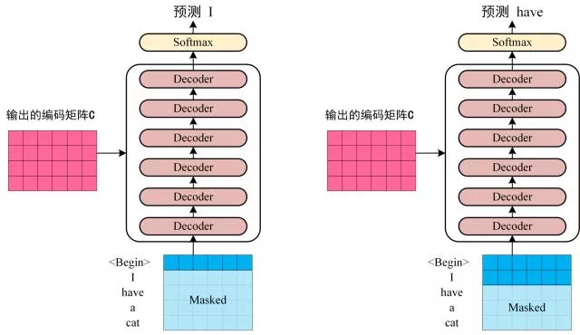
第三步：将编码器输出的编码信息矩阵 C 传递到解码器中，解码器会根据当前翻译过的单词 1~ i 依次翻译下一个单词 i+1，如下图所示：

Self-Attention 机制

下图展示了 Self-Attention 的结构。在计算时需要用到 Q(查询), K(键值), V(值)。在实践中，Self-Attention 接收的是输入（单词表示向量 x 组成的矩阵 X）或者上一个 Encoder block 的输出。而 Q, K, V 正是基于 Self-Attention 的输入进行线性变换得到的。

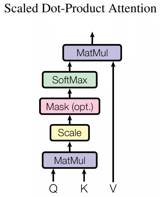
那么 Self-Attention 如何实现呢？

让我们来看一个具体的例子（以下示例图片来自博客 https://jalammar.github.io/illustrated-transformer/）。

假如我们要翻译一个词组 Thinking Machines，其中 Thinking 的词向量用 x1 表示，Machines 的词向量用 x2 表示。

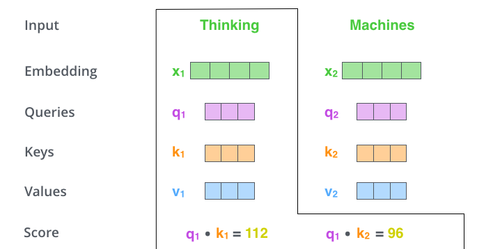
当处理 Thinking 这个词时，需要计算它与所有词的 attention Score，将当前词作为 query，去和句子中所有词的 key 匹配，得出相关度。用 q1 代表 Thinking 对应的 query vector，k1 及 k2 分别代表 Thinking 和 Machines 的 key vector。在计算 Thinking 的 attention score 时，需要先计算 q1 与 k1 及 k2 的点乘，同理在计算 Machines 的 attention score 时也需要计算 q_2 与 k1 及 k2 的点乘。如上图得到了 q1 与 k1 及 k2 的点乘，然后进行尺度缩放与 softmax 归一化，得到：

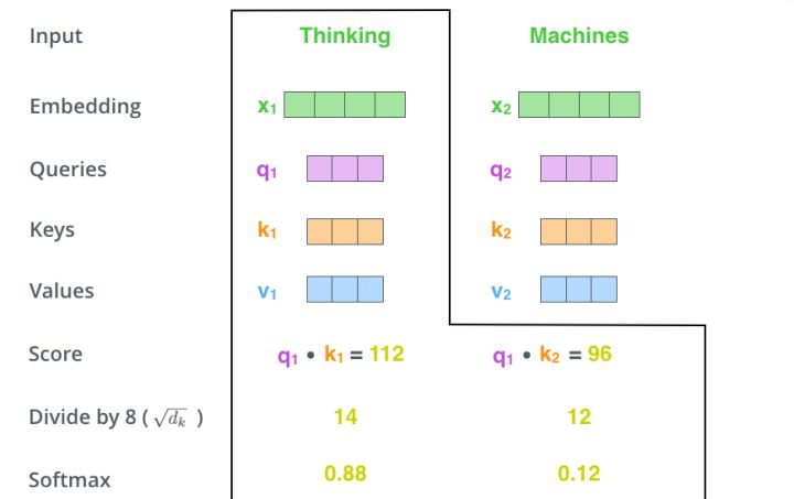
显然，当前单词与其自身的 attention score 最大，其他单词根据与当前单词的重要程度得到相应的 score。然后再将这些 attention score 与 value vector 相乘，得到加权的向量。

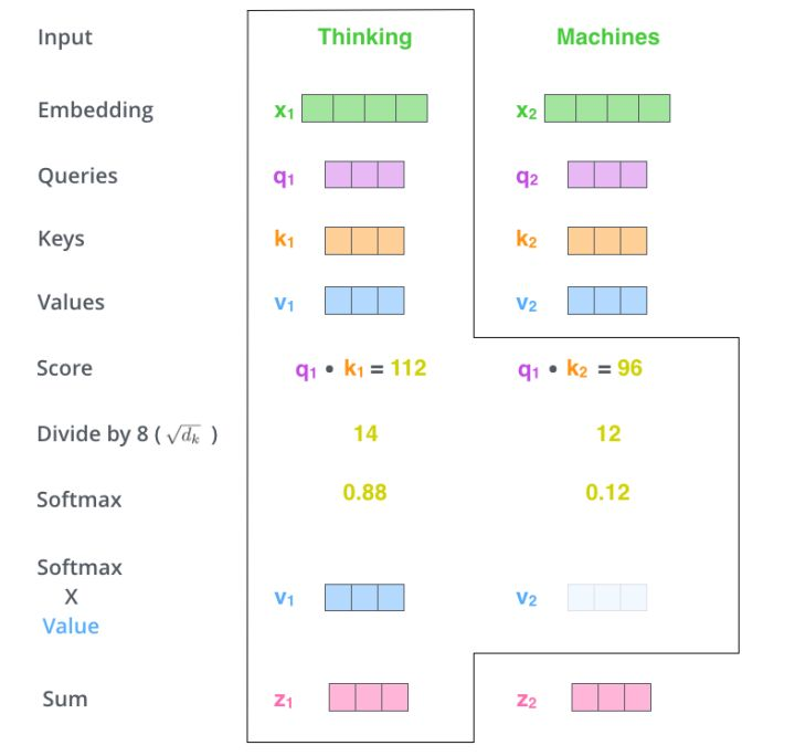
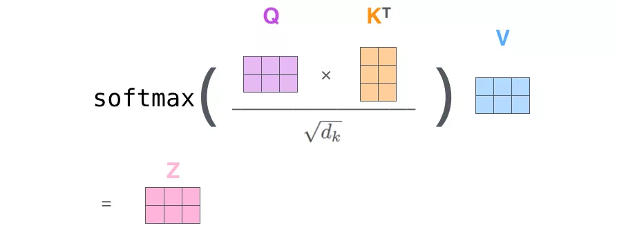
如果将输入的所有向量合并为矩阵形式，则所有 query, key, value 向量也可以合并为矩阵形式表示。以上是一个单词一个单词的输出，如果写成矩阵形式就是 Q*K，经过矩阵归一化直接得到权值。

原始Transformer结构

原始的Transformer 采用Encoder-Decoder 架构，其包含Encoder 和Decoder 两部分。这两部分都是由自注意力模块和全连接前馈模块重复连接构建而成。其整体结构如图1.7所示。

其中，Encoder 部分由六个级联的encoder layer 组成，每个encoder layer 包含一个注意力模块和一个全连接前馈模块。其中的注意力模块为自注意力模块（query，key，value 的输入是相同的）。Decoder 部分由六个级联的decoder layer 组成，每个decoder layer 包含两个注意力模块和一个全连接前馈模块。

其中，第一个注意力模块为自注意力模块，第二个注意力模块为交叉注意力模块（query，key，value 的输入不同）。Decoder 中第一个decoder layer 的自注意力模块的输入为模型的输出。其后的decoder layer 的自注意力模块的输入为上一个decoder layer 的输出。Decoder 交叉注意力模块的输入分别是自注意力模块的输出（query）和最后一个encoder layer 的输出（key，value）。

Transformer构造模块

Transformer 是由两种模块组合构建的模块化网络结构。两种模块分别为：（1）注意力（Attention）模块；（2）全连接前馈（Fully-connected Feedforwad）模块。其中，自注意力模块由自注意力层（Self-Attention Layer）、残差连接（Residual Connections）和层正则化（Layer Normalization）组成。全连接前馈模块由全连接前馈层，残差连接和层正则化组成。两个模块的结构示意图如图1.5所示。

以下详细介绍每个层的原理及作用。

1. 注意力层（Attention Layer）

注意力层采用加权平均的思想将前文信息叠加到当前状态上。Transformer 的注意力层将输入编码为query，key，value 三部分，即将输入{x1, x2, ..., xt} 编码为{(q1, k1, v1), (q2, k2, v2), ..., (qt, kt, vt)}。其中，query 和key 用于计算自注意力的权重α, value 是对输入的编码。Transformer 自注意力的实现图1.6所示。

上图中，the output of the attention layer is O3 which the attention of the input sententice {x1, x2, x3}, writing as Attention(x） , 具体计算如下：

2. 全连接前馈层（Fully-connected Feedforwad Layer）

全连接前馈层占据了Transformer 近三分之二的参数，掌管着Transformer 模型的记忆。其可以看作是一种Key-Value 模式的记忆存储管理模块。全连接前馈层包含两层，两层之间由ReLU 作为激活函数。设全连接前馈层的输入为v, 全连接前馈层可由下式表示：

FFN(v) = max(0,W1v + b1)W2 + b2

其中，W1 和W2 分别为第一层和第二层的权重参数，b1 和b2 分别为第一层和第二层的偏置参数。其中第一层的可看作神经记忆中的key，而第二层可看作value。

3. 层正则化（Layer Normalization）

层正则化用以加速神经网络训练过程并取得更好的泛化性能[1]。设输入到层正则化层的向量为v = (v1,v2,...,vn)，层正则化层将在v 的每一维度vi 上都进行层正则化操作。具体地，层正则化操作可以表示为下列公式：

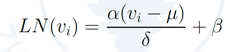
其中，α 和β 为可学习参数。μ 和δ 分别是隐藏状态的均值和方差，可由下列公式分别计算。

4. 残差连接（Residual Connections）

引入残差连接可以有效解决梯度消失问题。在基本的Transformer 编码模块中包含两个残差连接。第一个残差连接是将自注意力层的输入由一条旁路叠加到自注意力层的输出上，然后输入给层正则化。第二个残差连接是将全连接前馈层的输入由一条旁路引到全连接前馈层的输出上，然后输入给层正则化。上述将层正则化置于残差连接之后的网络结构被称为Post-LN Transformer。与之相对的，还有一种将层正则化置于残差连接之前的网络结构，称之为Pre-LNTransformers。对比两者，Post-LN Transformer 应对表征坍塌（Representation Collapse）

的能力更强，但处理梯度消失略弱。而Pre-LN Transformers 可以更好的应对梯度消失，但处理表征坍塌的能力略弱。

多头注意力（multi-head attentions）

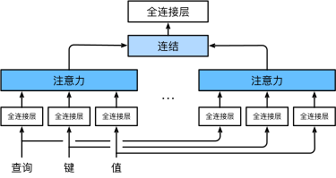
在实践中，当给定相同的查询、键和值的集合时， 我们希望模型可以基于相同的注意力机制学习到不同的行为， 然后将不同的行为作为知识组合起来， 捕获序列内各种范围的依赖关系 （例如，短距离依赖和长距离依赖关系）。 因此，允许注意力机制组合使用查询、键和值的不同 子空间表示（representation subspaces）可能是有益的。

为此，与其只使用单独一个注意力汇聚， 我们可以用独立学习得到的$h$组不同的 线性投影（linear projections）来变换查询、键和值。 然后，这$h$组变换后的查询、键和值将并行地送到注意力汇聚中。 最后，将这$h$个注意力汇聚的输出拼接在一起， 并且通过另一个可以学习的线性投影进行变换， 以产生最终输出。 这种设计被称为多头注意力（multihead attention） (Vaswani et al., 2017)。 对于$h$个注意力汇聚输出，每一个注意力汇聚都被称作一个头（head）。 图10.5.1 展示了使用全连接层来实现可学习的线性变换的多头注意力。

多头注意力：多个头连结然后线性变换

3. Transformer 语言模型

语言模型的输出为一个向量，该向量的每一维代表着词典中对应词的概率。在采用自回归范式的文本生成任务中，语言模型将依次生成一组向量并将其解码为文本。将这组向量解码为文本的过程被成为语言模型解码。

Top-P 随机采样方法

Top-P 方法可以克服生产文本“胡言乱语”和“枯燥无趣”。

为Top-p采用添加Temperature

Temperature 机制通过对Softmax函数中的自变量进行尺度变换，然后利用Softmax 函数的非线性实现对分布的控制。设Temperature 尺度变换的变量为T，引入Temperature 后，Top-P 采样的候选集的分布如下所示：

容易看出，当T > 1 时，Temperature 机制会使得候选集中的词的概率差距减小，分布变得更平坦，从而增加随机性。当0 < T < 1 时，Temperature 机制会使得候选集中的元素的概率差距加大，强者越强，弱者越弱，概率高的候选词会容易被选到，从而随机性变弱。Temperature 机制可以有效的对随机性进行调节来满足不同的需求。

涌现能力（Emergent Abilities）

如图2.2所示，模型训练数据规模以及参数数量的不断提升，不仅带来了上述学习能力的稳步增强，还为大模型“解锁”了一系列新的能力4，例如上下文学习能力、常识推理能力、数学运算能力、代码生成能力等。值得注意的是，这些新能力并非通过在特定下游任务上通过训练获得，而是随着模型复杂度的提升凭空自然涌现。这些能力因此被称为大语言模型的涌现能力（Emergent Abilities）。

• 上下文学习能力
• 常识推理能力
• 数学运算能力
• 代码生成能力
• 多模态理解能力

Stock Option Aide 2024.12

Stock Option Aide is a cross-platform version of Option Calculator app, I have to rename it because the app with the same name has existed on Apple Store.

1. Release Notes

• It can run on Windows, Android, iOS and Mac OS.
• It can use free Yahoo Finance data without account.
• It can use Schwab market data (need Schwab brookerage account).
• Bug fixes

2. Installation

• Android

        Click here to download and install it on your Android mobile.

• Win10-x64

1. Click StockOptionAide_2024.12.11.0_x64.zip to download zip file.
2. Unzip it to a temporary directionary
3. Double click the .cer file to install certificate if it is the first time to install this app. You should select to install certificate to Local Machine -> Certificate store: Trusted Person.
4. Double click the .msix file to install application.

• Win10-arm64

1. Click StockOptionAide_2024.12.11.0_arm64.zip to download zip file.
2. Unzip it to a temporary directionary
3. Double click the .cer file to install certificate if it is the first time to install this app. You should select to install certificate to Local Machine -> Certificate store: Trusted Person.
4. Double click the .msix file to install application.

• iOS

        hold on...

• MacOS

        hold on...

3. Where are the data from?

Yahoo Finance

The first time when the app starts on, it chooses Yahoo Finance for free stock data that has 15 minutes delay. 

Schwab real-time data

If you have a Schwab brookerage account already, you can switch to Schwab to use real-time market data. Click top-left menu -> select Data -> select Schwab -> click "Create Key", and then follow the instruction to create key to access Schwab data.

When first time to create the key, the instruction should guide you through how to create a Schwab Trade API developer account and create your app under your developer account, this is required by Schwab and it is only one time work. Schwab will spend a few days to verify and authenticate your application. Once it is authenticate, you will need to come back to this screen again to continue the rest of the steps to complete key creation.

4. How to understand the charts?

Reference the old app Option Calculator 3.0.0.

CompileTimeWeaver.Fody 3.3.3

 

Compile Time Weaver for AOP implementation

1. Introduce

NuGet package: https://www.nuget.org/packages/CompileTimeWeaver.Fody

DotNet Platform: NetStandard 2.0

Installation: 

PM> Install-Package CompileTimeWeaver.Fody

Different from runtime interception with dynamic proxy, this tool rewrites assembly at compile time, so that your code get these achievements that dynamic proxy based enhancement cannot give:

• Much better performance, no dynamic proxy, no thread block or reflection at run time.
• Directly instantiate your weaved classes with C# "new" operator
• weave virtual methods/properties
• weave static methods/properties
• weave  extension methods
• weave constructors
• Add property changed notification to auto-properties

2. Advice Based Programming Model

Start with version 2, this tool support advice based programming model. Advice based programming model has these superiorities comparing to the old decorator based programing model in version 1:

• Easy to intercept async method without thread blocking
• Simple to control the flow and add “before”, “after”, “around” and “exception” advices
• Allow to advise methods with parameters of reference type, value type and generic type, ref parameters and out parameters are allowed, too.

2.1. Step-by-step Instruction

Step 1) Create a C# project with VisualStudio.Net
Step 2) Install nuget package CompileTimeWeaver.Fody

Install NuGet package from https://www.nuget.org/packages/CompileTimeWeaver.Fody, you will see a FodyWeavers.xml file is added into project. The FodyWeavers.xml file content should have "CompileTimeWeaver" node as below, add it manually if the CompileTimeWeaver node is missing.

<?xml version="1.0" encoding="utf-8"?>
<Weavers>
  <CompileTimeWeaver />
</Weavers>

Step 3) Add MyAdvice class as below

using CompileTimeWeaver;
public class MyAdvice : AdviceAttribute
{
    public override object Advise(IInvocation invocation)
    {
        // do something before target method is Called
        // ...
        Trace.WriteLine("Entering " + invocation.Method.Name);

        try
        {
            return invocation.Proceed();    // call the next advice in the "chain" of advice pipeline, or call target method
        }
        catch (Exception e)
        {
            // do something when target method throws exception
            // ...
            Trace.WriteLine("MyAdvice catches an exception: " + e.Message);
            throw;
        }
        finally
        {
            // do something after target method is Called
            // ...
            Trace.WriteLine("Leaving " + invocation.Method.Name);
        }
    }

    public override async Task<object> AdviseAsync(IInvocation invocation)
    {
        // do something before target method is Called
        // ...
        Trace.WriteLine("Entering async " + invocation.Method.Name);

        try
        {
            return await invocation.ProceedAsync(); // asynchroniously call the next advice in the "chain" of advice pipeline, or call target method
        }
        catch (Exception e)
        {
            // do something when target method throws exception
            // ...
            Trace.WriteLine("MyAdvice catches an exception: " + e.Message);
            throw;
        }
        finally
        {
            // do something after target method is Called
            // ...
            Trace.WriteLine("Leaving async " + invocation.Method.Name);
        }
    }
}

Step 4) Add [MyAdvice] to any of your class on class level or method level. 

In the example below, [MyAdvice] is applied on MyClass class, and MyAdvice and MyClass can be in different assemblies.

[MyAdvice]
public class MyClass
{
    public int Add(int x, int y)
    {
        return x + y;
    }

    public Task<int> AddAsync(int x, int y)
    {
        await Task.Delay(1000);
        return x + y;
    }
}

That is it. You don't need dynamic proxy such as Castle DynamicProxy, directly use you class as usual in C#, for example:

var obj = new MyClass();
int z = obj.Add(1, 2);

z = await obj.AddAsync(1,2);

The first time when you compile your project, FodyWeavers.xml and FodyWeavers.xsd are generated if they do not exist yet. The FodyWeavers.xml file content should have "CompileTimeWeaver" node as below, add it manually if the CompileTimeWeaver node is missing.

<?xml version="1.0" encoding="utf-8"?>
<Weavers>
  <CompileTimeWeaver />
</Weavers>

Debug your code, you will see your Add() method and AddAsync() method have been magically rewritten, and the output is as below:

Entering .ctor...
Leaving .ctor...
Entering Add...
Leaving Add...
Entering AddAsync...
Leaving AddAsync...

2.2. Advice class specification

• Inherits AdviceAttribute class, or
• Inherits Attribute class and implements IAdvice interface

2.3. Rules

• When multiple advices are applied to a method, the advices are invoked as a pipe line, the Advise() or AdviseAsync() of the first advice is called first.
• When an advice is applied to class level, it is identical to this advice is added on each constructor and each method.
• Class level advices appears before all constructor/method level advices
• Each advice is assigned an Order, it is the sequence number of the appearance in the type group.
• Each advice on a recursive method is invoked only when the method was entered at the very first time, re-entrances don’t invoke the advice again, for performance reason.

3. Built-in advices

There are some built-in advices that you can immediately take advantage in your code, they are listed here.

3.1. NotifyPropertyChangedAttribute

When NotifyPropertyChangedAttribute is applied to a class, the class automatically implements INotifyPropertyChanged interface (if it is not implemented) and the setters of auto properties fire PropertyChanged event when the property values change.

If you do not want a specific setter to fire event, just apply IgnoreNotifyPropertyChangedAttribute to the property, and the setter will not be rewritten.

[NotifyPropertyChanged]
public class MyClass //: INotifyPropertyChanged - optional
{
    //public event PropertyChangedEventHandler PropertyChanged; - optional

    public string Name { get; set; }
    public int Age { get; set; }

    [IgnoreNotifyPropertyChanged]
    public string Password { get; set; }
}

One property change may cause the other property changes, DeterminedByPropertiesAttribute is to define dependancy relations between properties. In the code below, the change of property A fires property change events for property A, C and D, too.

[NotifyPropertyChanged]
public class MyClass //: INotifyPropertyChanged - optional
{
    public int A { get; set; }
    public int B { get; set; }

    [DeterminedByProperties("A")]
    public int C => A + 1;

    [DeterminedByProperties("B","C")]
    public int D => B + C;
}

3.2. LoggingAttribute

When LoggingAttribute is applied to a class or a method, the parameters of the constructor and methods are written into NLog, Log4Net or Serilog, depending on what logging package is enabled. [IgnoreLogging] is used to disable sensitive parameter logging. For example:

[Logging]
public class ClassWithLog
{
    public static void MethodWithLog(
		string userName,
		[IgnoreLogging]string password,
		int x,
		int y)
    {
        ...
    }

    [IgnoreLogging]
    public static int MethodWithoutLog(int x, int y)
    {
        ...
    }
}

//The example application using Serilog calls ClassWithLog
using Serilog;
    
class Program
{
    static void Main(string[] args)
    {
        Serilog.Log.Logger = new Serilog.LoggerConfiguration()
                                .MinimumLevel.Debug()
                                .Enrich.FromLogContext()
                                .WriteTo.Console()
                                .CreateLogger();

        ClassWithLog.MethodWithLog("Simon", "fdhasdewjsdfsdfe", 1, 2);
        ClassWithLog.MethodWithoutLog(1, 2);

        Serilog.Log.CloseAndFlush();
    }
}

When ClassWithLog.MethodWithLog method is called, you will see log messages as below, parameter values in log are from their ToString() method, and password parameter is not logged because of [IgnoreLogging] on it.

MethodWithLog...
        userName: Simon
        x: 1
        y: 2
MethodWithLog completed in 5 milliseconds.

When ClassWithLog.MethodWithoutLog method is called, nothing is logged because it is decorated with [IgnoreLogging].

3.3. ExceptionHandlerAttribute

ExceptionHandler Attribute is an advice to consolidate exception handling logic into specific classes according to the exception types. In the example code below, the ApplicationExceptionHandler class defines ApplicationException handling logic and the IOExceptionHandler class defines IOException hanlding logic, you simply add ExceptionHandler decorations on the methods (HelloAsync as example below) to intercept the exceptions.

public class MyClass
{
    [ExceptionHandler(typeof(ApplicationException), typeof(ApplicationExceptionHandler))]
    [ExceptionHandler(typeof(IOException), typeof(IOExceptionHandler))]
    public async Task<int> HelloAsync()
    {
        await Task.Delay(1).ConfigureAwait(false);
        ...
        throw new ApplicationException();
        ...
        throw new IOException();
    }
}

internal class ApplicationExceptionHandler : IExceptionHandler
{
    public bool HandleException(Exception e)
    {
        Trace.WriteLine(e.GetType() + " is caught");
        return false;
    }
}

internal class IOExceptionHandler : IExceptionHandler
{
    public bool HandleException(Exception e)
    {
        Trace.WriteLine(e.GetType() + " is caught");
        return false;
    }
}

Option Calculator 3.0.0

Share is care!

Option Calculator 3.0.0 is shared with all my friends today after a long time waiting.

1. Release Notes

• Improved IV calculation algorithm.
• Added strike predication trend chart.
• Changed put/call skew calculation algorithm to be similar to that on fdscanner.com (see explanation below).
• Added PCR trend chart (see explanation below).
• Added correlation to inverted-UVXY
• Bug fixes

2. Installation

The App doesn't need installation, just click App on google drive, and download the correct file for your specific platform, save it on your local drive, double click it to start up.

If it is the first time you start up the app, it will ask you to download and install DotNet 5.0 Desktop Runtime from Microsoft website if it has not been installed yet.

3. Analysis Screen

Select a ticker that is exactly the same as it on yahoo finance, or enter the ticker and hit Enter key,

you will see the analysis screen as below. You can adjust sigma scale to see different sigma values.

Notes: 

• App only accept Yahoo Finance tickers, for example, "^SPX" rather than "SPX".
• EM means Expected Movement, it is expected market price change when sigma scale is one.
• The chart is spitted into 3 different areas by three X-axes: date, probability and premium.
• Candlesticks area

use mouse to drag and move the candlestick chart

scroll mouse wheel to zoom chart.

• Probability area 

shows the probabilities of call/put on each point, you can move mouse to the point to display the probability the market hits it.

• Premium area

shows the theoretical price of your option at each point, you can move mouse to it to display the premium.

• Solid horizontal line is the current market price.
• Thick green horizontal line is the call strike at 2 sigma.
• Thick red horizontal line is the put strike at 2 sigma.
• Thin green horizontal line is the call strike at 1 sigma.
• Thin red horizontal line the put strike at 1 sigma
• Blue horizontal line is the max pain point.

Analysis Screen

4. Let App Monitor Your Options for You.

You don't need to set it up if you don't want to receive alarms from this app, if you do want it to warn you by sending emails so that your phone can pop up alerts while you are playing golf, click the Setup button.

In the Setup button, you can input your own email address as sender and receiver so that you send alerts from yourself to yourself. Only Hotmail, Gmail and yahoo mail are supported so far.

Add the tickers you want the app to monitor for you, enter sigma scale and midpoint limit, etc., and click Save button.

Alarm Setup Screen

Notes:

• Midpoint is the point where the market has 50% chance to hit. You are suggested to set the midpoint limit to be your option strike, so that you will receive alert once the possibility of win or lose is break even.
• You can disable monitoring an option by set its midpoint limit to zero.
• If you leave midpoint empty (zero is not empty), app will automatically set midpoint to 2-sigma strike price when you click Save button.
• You can select the expiration date of the option you want it to monitor, empty expiration means the nearest valid expiry.

5. IV Trend

Implied volatility (IV) is denoted by the symbol σ (sigma). It can often be thought to be a proxy of market risk, it is expressed using percentages and standard deviations over a specified time horizon. My app calculates IV with Black-Scholes option model.

Trend Charts Screen

6. What is Put/Call Skew?

On fdscanner.com, put/call skew is defined as the price of 10% OTM puts/10% OTM calls on option expiry. A put skew of 2.1 means the 10% OTM put is 2.1x the price of 10% OTM call. There are often underlying reasons worth researching before entering option position for stocks with high/low skew.

Theoretically, an equally OTM put and call trades at the same price after accounting for cost of carry, dividends and shorting costs. However, the real world doesn't always follow theory. Demand supply imbalances do happen and below are some possible reasons.

• Institutions using the Collar strategy, buying puts and selling calls to limit downside at the cost of upside.
• High demand/Low supply for puts, driving up put prices. Usual occurrence during bear markets.
• Low demand/High supply for calls, driving down calls prices.
• Stock had recent huge upward price movements and is grossly overvalued, shifting the supply/demand curve for puts.
• Dividends contributes to put skew, especially if the dividend is a large percentage of stock price.

Computing the Put/Call Skew

Calculating the skew requires 4 option prices, the 2 put options surrounding 90% current share price, and the 2 call options surrounding 110% of current share price. All 4 of these options must have bid/ask spread of below 25% to be included in the Put/Call Skew Index.

Example Computation

In this example, MA had a put skew of 1.911, let's see how this number is computed from raw data.

Step 1: Computing prices, getting the right strikes

Legend	Description	Computation	Output
Price	Current Share Price		$269.16
110% SP	110% of Current Share Price	$269.16 * 1.1	$296.08
90% SP	90% of Current Share Price	$92 * 0.9	$242.24
High Call Strike	Call option immediately above 110% SP	Strike above $296.08	$300 Call
Low Call Strike	Call option immediately below 110% SP	Strike below $296.08	$295 Call
High Put Strike	Put option immediately above 90% SP	Strike above $242.24	$245 Put
Low Put Strike	Put option immediately below 90% SP	Strike below $242.24	$240 Put

Step 2: Ensuring options pass liquidity checks

Option	Expiry	Bid	Ask	Ask/Bid
$295 Call	6/19	$2.64	$2.93	2.93/2.64 ~= 1.11
$300 Call	6/19	$1.65	$1.97	1.97/1.65 ~= 1.19
$240 Put	6/19	$4.30	$4.60	4.6/4.30 ~= 1.07
$245 Put	6/19	$5.20	$5.75	5.75/5.20 ~= 1.10

The liquidity check requires Ask/Bid of all 4 options to be below 1.25. If any are above 1.25, they are excluded from Put/Call Skew index. Stocks that barely make the liquidity cut off may enter and exit the Put/Call Skew index multiple times per day.

Step 3: Computing option midpoints

Option	Computation	Midpoint price
$295 Call	(2.64 + 2.93)/2	$2.79
$300 Call	(1.65 + 1.97)/2	$1.81
$240 Put	(4.3 + 4.6)/2	$4.45
$245 Put	(5.2 + 5.75)/2	$5.48

The midpoint price is taken as the price for that option.

Step 4: Interpolated Price

Option	Computation	Interpolated price
$296.08 Call	2.785 - (2.785-1.81)/(300-295) * (296.08 - 295)	$2.57
$242.24 Put	4.45 + (5.475-4.45)/(245-240) * (242.24 - 240)	$4.90

Interpolate between the midpoint price of the 2 call and put options.

Step 5: Calculate Skew

Put interpolated price/call interpolated price, 4.898/2.5744 = 1.903. If the Put price is higher, the skew value is greater than 1. If Call price is higher, the skew is less than 1.

Notice: In my app, put/call skew is defined as the price of 5% OTM puts/the price of 5% OTM calls on option expiry, rather than 10% OTM as fdscanner does.

7. Strike Trend

The strike trend in the above screenshot is a predication of a stock price. The app display Max Pain trend and a few predication prices in the chart.

First, the app calculates the max-pain point of the stock on each expiry, to indicate the rough market movement. To predicate market with max pain sometimes works well on large cap ETFs, such as SPX and QQQ, that are not easy to manipulate by individual institute.

Second, the app use a prediction model to predict the next 5 trading days of the stock prices, please see the prediction lines in app screen.

8. What is PCR?

PCR is the abbreviation of put call ratio, there are two kinds of PCRs: PCR(OI) and PCR(Volume).

PCR(OI) = sum of open interests of put options on a given day/sum of open interests of call options on the same given day.

PCR(Vol) = sum of volumes of put options on a given day/sum of volumes of call options on the same given day.

How to interpret the Put Call Ratio to take a view on markets
If you browse through any derivatives report put out by a broker, you will find a lot of emphasis on the PCR. So, how exactly do you interpret the Put Call ratio in practical terms?

One of the most important things that you need to understand is that the PCR is normally used as a popular contrarian indicator. That means the conclusions are actually counterintuitive. Let us understand this point in greater detail. There is nothing like a range for PCR or an ideal level for PCR. It is the trend that is more important. Here are a few key pointers pertaining to PCR interpretation..

Normally, times of greed and fear are reflected by significantly high or significantly low levels of PCR. Contrarians believe that PCR is normally headed in the wrong direction when markets are overbought or oversold and that becomes a key guiding factor.

Let us assume that the PCR has gone up sharply in the last few days and the market index has also corrected by 15% during the last 1 month. How do we interpret this situation? Contrarians believe that there is too much pessimism as small and retail investors are just buying too much of puts to hedge their downside risk. In any F&O market, the put writing is typically done by savvy traders and institutions. High PCR means aggressive put buying by small and medium investors but it also means aggressive selling by more savvy traders. Typically savvy traders sell only when they believe that downside is limited. That could be an indication that markets are bottoming out.

The reverse situation holds when markets have shot up and the PCR is falling. It means small and medium investors are heavily buying into calls but it also means that savvier investors are selling calls. That is an indication that markets may be topping out.

Combining PCR with Implied volatility (IV)
A smart way of interpreting PCR is by combining it with IV. Remember, IV is the volatility that is implied in the option price and it reflects the risk perception in the market. Here are a few pointers..

If the PCR increases with an increase in IV, it indicates that the put activity is increasing with a heightened sense of risk. That is a bearish signal.

If the PCR increases with a decrease in IV, it indicates that put activity is increasing with a falling sense of risk. That means more writing of puts and is a bullish signal.

If the PCR decreases with decrease in IV, it is indicative of unwinding of Puts and can be interpreted as a signal that markets may be bottoming out.

If the PCR decreases with an increase in IV, it means that puts are just being covered and the markets will again fall once the covering is done with.

9. Correlation to Inverted-UVXY

If UVXY is trader's fear gauges, the inverted-UVXY is peace gauges. Let's say you want to see the correlation between QQQ and inverted-UVXY, you can select QQQ in the ticker drop down list and then select "1 month/day" as data granularity, and you will be able to see a correlation coefficient chart as below.

Correlation to Inverted-UVXY

A correlation coefficient is a value between -1 and +1, when it is near 0, QQQ has low correlation to inverted-UVXY; when it is close to +1, they are positively correlated; when it is close to -1, they are negatively correlated. 

Acknowledgement

I give thanks to everyone who has shared their knowledges with me and has supported me to develop this app. I am glad if this app is useful for you, and appreciate it if you send me a cup of coffee by click the PayPal Donate button below.